Noch nich översett

Disse Sied is noch nich översett. Se kiekt de engelsche Originalversion an.

Operator backpropagation (OBP)

Operator backpropagation (OBP) is a technique to reduce circuit depth by trimming operations from its end at the cost of more operator measurements. There are a number of ways in which operator backpropagation can be performed, and this package uses a method based on Clifford perturbation theory [1].

As one propagates an operator further through a circuit, the size of the observable to measure grows exponentially. This results in both a classical and quantum resource overhead. However, for some circuits, the resulting distribution of additional Pauli observables is more concentrated than the worst-case exponential scaling. This implies that some terms in an observable with small coefficients can be truncated to reduce the quantum overhead. The error incurred by doing so can be controlled to find a suitable tradeoff between precision and efficiency.

Installation

You can install the OBP package in one of two ways: via PyPI or building from source. Consider installing these packages in a virtual environment to ensure separation between package dependencies.

Install from PyPI

The most straightforward way to install the qiskit-addon-obp package is via PyPI.

pip install qiskit-addon-obp

Build from source

Users who wish to contribute to this package or who want to install it manually may do so by first cloning the repository:

git clone git@github.com:Qiskit/qiskit-addon-obp.git
```_

and install the package via `pip`. The repository also contains example notebooks. If you plan on developing in the repository, install the `dev` dependencies.

Adjust the options to suit your needs:

```bash
pip install tox notebook -e '.[notebook-dependencies, dev]'

Theoretical background

The OBP procedure implemented in this package is described in detail in [1]. When using the Estimator primitive, the output of a quantum workload is the estimation of one or more expectation values $\langle O \rangle$ with respect to some state prepared using a QPU. This section summarizes the procedure.

First, start by writing the expectation value measurement of an observable $O$ in terms of some initial state $|\psi\rangle$ and a quantum circuit $U_Q$:

$\langle O \rangle_{U|\psi\rangle} = \langle\psi | U^\dagger O U |\psi \rangle.$

To distribute this problem across both classical and quantum resources, split the circuit $U$ into two subcircuits, $U_C$ and $U_Q$, classically simulate the circuit $U_C$, then execute the circuit $U_Q$ on quantum hardware and use the results of the classical simulation to reconstruct the measurement of the observable $O$.

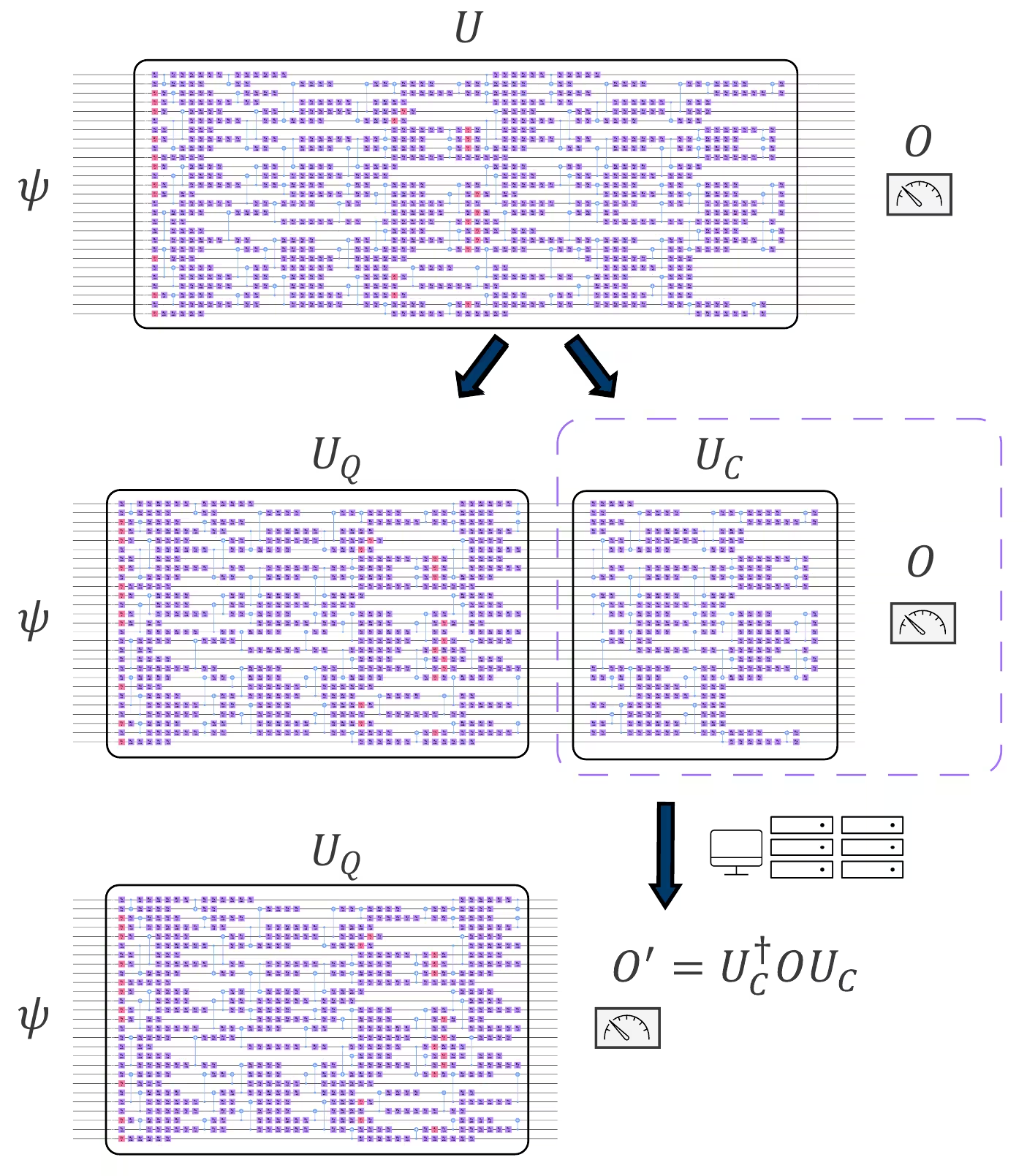
The subcircuit $U_C$ should be selected to be classically simulable and will compute the expectation value

$\langle O' \rangle \equiv U_C^\dagger O U_C,$

which is the version of the initial operator $O$ evolved through the circuit $U_C$. Once $O'$ has been determined, the quantum workload is prepared wherein the state $|\psi\rangle$ is initiated, has the circuit $U_Q$ applied to it, and then measures the expectation value $O'$. You can show that this is equivalent to measuring $\langle O \rangle$ by writing:

$\langle \psi | U_Q^\dagger O' U_Q \psi \rangle = \langle \psi | U_Q^\dagger U_C^\dagger O U_CU_Q \psi \rangle = \langle\psi | U^\dagger O U |\psi \rangle = \langle O \rangle_{U|\psi\rangle}$

Lastly, in order to measure the expectation value $\langle O' \rangle$, we must require it to be decomposable into a sum of Pauli strings

$O' = \sum_P c_P P,$

where $c_P$ are real coefficients of the decomposition and $P$ is some Pauli string composed of $I$, $X$, $Y$, and $Z$ operators. This ensures that you can reconstruct the expectation value of $O$ by

$\langle \psi | U_Q^\dagger O' |\psi \rangle = \sum_P c_P \langle \psi | U_Q^\dagger P U_Q | \psi \rangle.$

Truncating terms

This scheme offers a tradeoff between the required circuit depth of $U_Q$, the number of circuit executions on quantum hardware, and the amount of classical computing resources needed to compute $O'$. In general, as you choose to backpropagate further through a circuit, the number of Pauli strings to measure as well as the error-mitigation overhead both grow exponentially (alongside the classical resources needed to simulate $U_C$).

Fortunately, the decomposition of $O'$ can often contain coefficients that are quite small and can be truncated from the final measurements used to reconstruct $O$ without incurring much error. The qiskit-addon-obp package possesses functionality to specify an error budget, which can automatically search for terms that can be truncated, to within some error tolerance.

Clifford perturbation theory

Lastly, the qiskit-addon-obp package approaches operator backpropagation based on Clifford perturbation theory. This method has the benefit that the overhead incurred by backpropagating various gates scales with the non-Cliffordness of $U_C$ (i.e. how much of U C is comprised of non-Clifford instructions).

This approach to OBP begins by splitting the simulated circuit, $U_C$, into slices:

$U_C = \prod_{s=1}^S \mathcal{U}_s = \mathcal{U}_S...\mathcal{U}_2\mathcal{U}_1,$

where $S$ represents the total number of slices and $\mathcal{U}_s$ denotes a single slice of the circuit $U_C$. Each of these slices are then analytically applied in sequence to measure the back propagated operator $O'$ and may or may not contribute to the overall size of the sum, depending on if the slice is a Clifford vs non-Clifford operation. If an error budget is allocated, truncation will then occur between the application of each slice.

Next steps

Recommendations

• Get started with OBP.
• Become familiar with the error mitigation techniques available in Qiskit Runtime.
• Read the tutorial on using OBP to improve expectation values.

References

[1] Fuller, Bryce, et al. "Improved Quantum Computation using Operator Backpropagation." arXiv:2502.01897 [quant-ph] (2025).